Fitting Normal Distribution on House Price Data

What we have to prove?

House Price of each house can be modeled as Normal distribution with 95% confidence.

Importing Library

                import pandas as pd
                import matplotlib.pyplot as plt
                import numpy as np
                import scipy.stats as st

Data

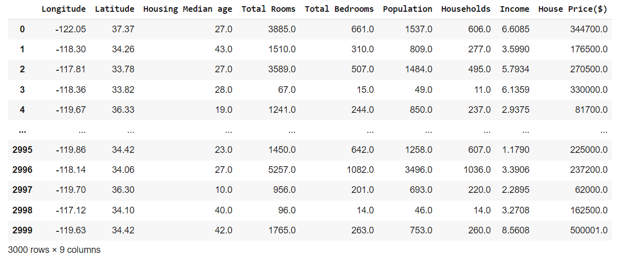
                d=pd.read_excel("/content/drive/MyDrive/Site Data/House Data.xlsx")
                d

                Output:-

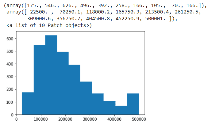
                plt.hist(d["House Price"],bins=10)

                Output:-

Simulation

* Fitting a Normal distribution

From the histogram, the distribution could be modelled as Normal$(\mu,\sigma^2)$. The next step is to estimate $\mu$ and $\sigma^2$ from the given samples.

* Method of Moments

Suppose $m_1$ and $m_2$ are the first and second moments of the samples. The method of moments estimates are obtained by solving $$m_1=\mu ,$$ $$m_2=\sigma^2+\mu^2.$$ The solution results in $$\hat{\mu}_{MM}=m_1,\hat{\sigma}_{MM}=\sqrt{m_2-m_1^2}.$$ We now compute the values of $m_1$ (sample mean) and $m_2-m_1^2$ (sample variance) from the data. After that, we can compute the estimates.

                x=np.array(d["House Price"])
                m1=np.average(x)
                ss=np.var(x)             # Computing sample variance.
                muMM = m1
                sigmaMM = ss**0.5       
                print(muMM)
                print(round(sigmaMM,3))

                Output:-
                μ : 205846.275
                σ : 113100.833

                
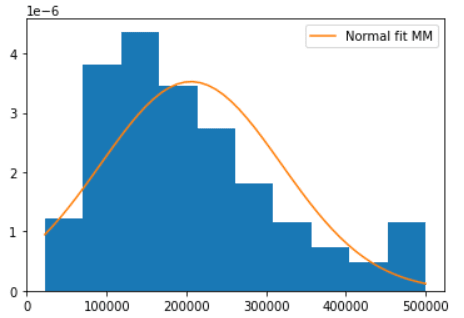
                # blue curve
                plt.hist(d["House Price"],bins=10,density=True)  

                # np.linespace(min,max,smooth)                                  
                domain= np.linspace(d["House Price"].min(),d["House Price"].max(),50)     
                
                # Orange Line.
                plt.plot(domain,st.norm.pdf(domain,loc=muMM,scale=sigmaMM),label='Normal fit MM')  
                plt.legend(loc='best')
                plt.show()

                Output:-

* Approximate confidence intervals with Bootstrap

> Bootstrap

How do we find the bias and variance of the estimator? Theoretical derivations of the sampling distributions may be too cumbersome and difficult in most cases. Bootstrap is a Monte Carlo simulation method for computing metrics such as bias, variance and confidence intervals for estimators.

In the above simulation, we have found $\hat{\mu}_{MM}=205846.275...$ and $\hat{\sigma}_{MM}=113100.833...$. Using these values, we simulate $n=1321$ iid samples from Normal$(205846.275...,113100.833...)$ and using the simulated samples, we compute new estimates of $\mu$ and $\sigma$ and call them $\hat{\mu}_{MM}(1)$ and $\hat{\sigma}_{MM}(1)$. Now, repeat the simulation $N$ times to get estimates $\hat{\mu}_{MM}(i)$ and $\hat{\sigma}_{MM}(i)$, $i=1,2,\ldots,N$.

> Confidence Intervals

Suppose a parameter $\theta$ is estimated as $\hat{\theta}$, and suppose the distribution of $\hat{\theta}-\theta$ is known. Then, to obtain $(100(1-\alpha))$% confidence intervals (typical values are $\alpha=0.1$ for 90% confidence intervals and $\alpha=0.05$ for 95% confidence intervals), we use the CDF of $\hat{\theta}-\theta$ to obtain $\delta_1$ and $\delta_2$ such that $$P(\hat{\theta}-\theta\le\delta_1)=1-\frac{\alpha}{2},$$ $$P(\hat{\theta}-\theta\le\delta_2)=\frac{\alpha}{2}.$$ Actually, the inverse of the CDF of $\hat{\theta}-\theta$ is used to find the above $\delta_1$ and $\delta_2$. From the above, we see that $$P(\hat{\theta}-\theta \le \delta_1)-P(\hat{\theta}-\theta \le \delta_2)= P(\delta_2< \hat{\theta}-\theta \le \delta_1)=1-\frac{\alpha}{2}-\frac{\alpha}{2}=1-\alpha.$$ The above is rewritten as $$P(\hat{\theta}-\delta_1\le\theta<\hat{\theta}-\delta_2)=1-\alpha,$$ and $[\hat{\theta}-\delta_1,\hat{\theta}-\delta_2]$ is interpreted as the $100(1-\alpha)$% confidence interval.

> Bootstrap confidence intervals

The CDF of $\hat{\theta}-\theta$ might be difficult to determine in many cases, and the bootstrap method is used often to estimate $\delta_1$ and $\delta_2$ for $\mu$.

We consider the list of numbers $\{\hat{\mu}_{MM}(1)-205846.275...,\ldots,\hat{\mu}_{MM}(N)-205846.275...\}$ and pick the $100(\alpha/2)$-th percentile and $100(1-\alpha/2)$-th percentile. Similarly we can estimate $\delta_1$ and $\delta_2$ for $\sigma$.

                N = 1000
                n = 1321
                mu_hat = np.zeros(N)
                sigma_hat = np.zeros(N)
                for i in np.arange(N):
                xi = st.norm.rvs(muMM,scale=sigmaMM,size=n)
                m1i = np.average(xi); ssi = np.var(xi)

                # Calculating mu_hat & sigma_hat with bootstrap.
                mu_hat[i] = m1i; sigma_hat[i] = ssi**0.5

                # del1 & del2 for μ.
                del1 = np.percentile(mu_hat - muMM, 95)
                del2 = np.percentile(mu_hat - muMM, 5)
                print([round(del1,3),round(del2,3)])

                Output:-
                [5140.216, -5027.517]

The 95% confidence interval for $\mu$ using the method of moments estimator works out to $[205846.275-5140.216, 205846.275-(-5027.517)] = [200706.059, 210873.792]$.

                # del1 & del2 for σ.
                dels1 = np.percentile(sigma_hat - sigmaMM, 95)
                dels2 = np.percentile(sigma_hat - sigmaMM, 5)
                print([round(dels1,3),round(dels2,3)])

                Output:-
                [3541.747, -3648.79]

The 95% confidence interval for $\sigma$ using the method of moments estimator works out to $[113100.833-3541.747, 113100.833-(-3648.79)] = [109559.086, 116749.623]$.

Conclusion

Hence, We can claim that House Price of each house can be modeled as Normal distribution with 95% confidence that

$\mu$ lies in $[200706.059, 210873.792]$ range and $\sigma$ lies in $[109559.086, 116749.623]$ range.

$Note:-$ I Use Python Programming Language for giving simulation.